- Pandas
- Installer Pandas
- Importer Pandas
- Créer une série Pandas avec l'index par défaut
- Créer une série Pandas avec un index personnalisé
- Créer une série Pandas à partir d'un dictionnaire
- Créer une série Pandas constante
- Créer une série Pandas avec Linspace
- DataFrames
- Lire un fichier CSV avec Pandas
- Modifier un DataFrame
- Vérifier les types de données des colonnes
- Exercices : Jour 25
Pandas
Pandas est une bibliothèque open source, haute performance et facile à utiliser, fournissant des structures de données et des outils d'analyse de données pour le langage de programmation Python. Pandas ajoute des structures de données et des outils conçus pour travailler avec des données tabulaires, à savoir les Series et les DataFrames. Pandas fournit des outils de manipulation de données :
- remaniement (reshaping)
- fusion (merging)
- tri (sorting)
- découpage (slicing)
- agrégation (aggregation)
- imputation (imputation) Si vous utilisez anaconda, vous n'avez pas besoin d'installer pandas.
Installer Pandas
Pour Mac :
pip install conda
conda install pandas
Pour Windows :
pip install conda
pip install pandas
La structure de données de Pandas est basée sur les Series et les DataFrames.
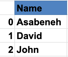
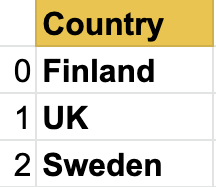
Une series est une colonne et un DataFrame est une table multidimensionnelle composée d'un ensemble de series. Pour créer une série pandas, nous devons utiliser numpy pour créer un tableau unidimensionnel ou une liste Python. Voyons un exemple de série :
Série Pandas des noms
Série des pays
Série des villes
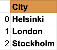
Comme vous pouvez le voir, une série pandas est juste une colonne de données. Si nous voulons avoir plusieurs colonnes, nous utilisons les data frames. L'exemple ci-dessous montre les DataFrames pandas.
Voyons un exemple de data frame pandas :
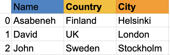
Un data frame est un ensemble de lignes et de colonnes. Regardez le tableau ci-dessous ; il a beaucoup plus de colonnes que l'exemple ci-dessus :
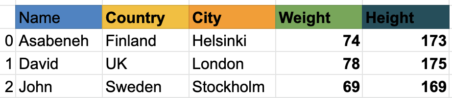
Ensuite, nous verrons comment importer pandas et comment créer des Series et des DataFrames avec pandas.
Importer Pandas
import pandas as pd # importation de pandas en tant que pd
import numpy  as np # importation de numpy en tant que np
Créer une série Pandas avec l'index par défaut
nums = [1, 2, 3, 4,5]
s = pd.Series(nums)
print(s)
    0    1
    1    2
    2    3
    3    4
    4    5
    dtype: int64
Créer une série Pandas avec un index personnalisé
nums = [1, 2, 3, 4, 5]
s = pd.Series(nums, index=[1, 2, 3, 4, 5])
print(s)
    1    1
    2    2
    3    3
    4    4
    5    5
    dtype: int64
fruits = ['Orange','Banana','Mango']
fruits = pd.Series(fruits, index=[1, 2, 3])
print(fruits)
    1    Orange
    2    Banana
    3    Mango
    dtype: object
Créer une série Pandas à partir d'un dictionnaire
dct = {'name':'Asabeneh','country':'Finland','city':'Helsinki'}
s = pd.Series(dct)
print(s)
    name       Asabeneh
    country     Finland
    city       Helsinki
    dtype: object
Créer une série Pandas constante
s = pd.Series(10, index = [1, 2, 3])
print(s)
    1    10
    2    10
    3    10
    dtype: int64
Créer une série Pandas avec Linspace
s = pd.Series(np.linspace(5, 20, 10)) # linspace(début, fin, éléments)
print(s)
    0     5.000000
    1     6.666667
    2     8.333333
    3    10.000000
    4    11.666667
    5    13.333333
    6    15.000000
    7    16.666667
    8    18.333333
    9    20.000000
    dtype: float64
DataFrames
Les data frames pandas peuvent être créés de différentes manières.
Créer des DataFrames à partir d'une liste de listes
data = [
    ['Asabeneh', 'Finland', 'Helsink'],
    ['David', 'UK', 'London'],
    ['John', 'Sweden', 'Stockholm']
]
df = pd.DataFrame(data, columns=['Names','Country','City'])
print(df)
Créer un DataFrame avec un dictionnaire
data = {'Name': ['Asabeneh', 'David', 'John'], 'Country':[
    'Finland', 'UK', 'Sweden'], 'City': ['Helsiki', 'London', 'Stockholm']}
df = pd.DataFrame(data)
print(df)
Créer des DataFrames à partir d'une liste de dictionnaires
data = [
    {'Name': 'Asabeneh', 'Country': 'Finland', 'City': 'Helsinki'},
    {'Name': 'David', 'Country': 'UK', 'City': 'London'},
    {'Name': 'John', 'Country': 'Sweden', 'City': 'Stockholm'}]
df = pd.DataFrame(data)
print(df)
Lire un fichier CSV avec Pandas
Pour télécharger le fichier CSV nécessaire dans cet exemple, la console ou la ligne de commande suffit :
curl -O https://raw.githubusercontent.com/Asabeneh/30-Days-Of-Python/master/data/weight-height.csv
Placez le fichier téléchargé dans votre répertoire de travail.
import pandas as pd

df = pd.read_csv('weight-height.csv')
print(df)
Exploration des données
Lisons seulement les 5 premières lignes avec head()
print(df.head()) # donne cinq lignes, on peut augmenter le nombre en passant un argument à head()
Explorons également les derniers enregistrements du dataframe avec la méthode tail().
print(df.tail()) # tail donne les cinq dernières lignes, on peut augmenter le nombre en passant un argument à tail()
Comme vous pouvez le voir, le fichier csv a trois colonnes : Gender, Height et Weight. Si le DataFrame avait beaucoup de lignes, il serait difficile de connaître toutes les colonnes. Par conséquent, nous devons utiliser une méthode pour connaître les colonnes. Nous ne connaissons pas non plus le nombre de lignes. Utilisons la méthode shape.
print(df.shape) # comme vous pouvez le voir, 10000 lignes et trois colonnes
(10000, 3)
Obtenons toutes les colonnes en utilisant columns.
print(df.columns)
Index(['Gender', 'Height', 'Weight'], dtype='object')
Maintenant, obtenons une colonne spécifique en utilisant la clé de la colonne
heights = df['Height'] # c'est maintenant une série
print(heights)
    0       73.847017
    1       68.781904
    2       74.110105
    3       71.730978
    4       69.881796
              ...
    9995    66.172652
    9996    67.067155
    9997    63.867992
    9998    69.034243
    9999    61.944246
    Name: Height, Length: 10000, dtype: float64
weights = df['Weight'] # c'est maintenant une série
print(weights)
    0       241.893563
    1       162.310473
    2       212.740856
    3       220.042470
    4       206.349801
              ...
    9995    136.777454
    9996    170.867906
    9997    128.475319
    9998    163.852461
    9999    113.649103
    Name: Weight, Length: 10000, dtype: float64
print(len(heights) == len(weights))
True
La méthode describe() fournit des valeurs statistiques descriptives d'un ensemble de données.
print(heights.describe()) # donne des informations statistiques sur les données de taille
    count    10000.000000
    mean        66.367560
    std          3.847528
    min         54.263133
    25%         63.505620
    50%         66.318070
    75%         69.174262
    max         78.998742
    Name: Height, dtype: float64
print(weights.describe())
    count    10000.000000
    mean       161.440357
    std         32.108439
    min         64.700127
    25%        135.818051
    50%        161.212928
    75%        187.169525
    max        269.989699
    Name: Weight, dtype: float64
print(df.describe()) # describe peut aussi donner des informations statistiques d'un DataFrame
De la même manière que describe(), la méthode info() donne aussi des informations sur l'ensemble de données.
Modifier un DataFrame
Modifier un DataFrame : * Nous pouvons créer un nouveau DataFrame * Nous pouvons créer une nouvelle colonne et l'ajouter au DataFrame, * nous pouvons supprimer une colonne existante d'un DataFrame, * nous pouvons modifier une colonne existante dans un DataFrame, * nous pouvons changer le type de données des valeurs d'une colonne dans le DataFrame
Créer un DataFrame
Comme toujours, nous importons d'abord les paquets nécessaires. Importons pandas et numpy, les deux meilleurs amis du monde.
import pandas as pd
import numpy as np
data = [
    {"Name": "Asabeneh", "Country":"Finland","City":"Helsinki"},
    {"Name": "David", "Country":"UK","City":"London"},
    {"Name": "John", "Country":"Sweden","City":"Stockholm"}]
df = pd.DataFrame(data)
print(df)
Ajouter une colonne à un DataFrame est comme ajouter une clé à un dictionnaire.
Utilisons d'abord l'exemple précédent pour créer un DataFrame. Après avoir créé le DataFrame, nous allons commencer à modifier les colonnes et leurs valeurs.
Ajouter une nouvelle colonne
Ajoutons une colonne weight dans le DataFrame
weights = [74, 78, 69]
df['Weight'] = weights
df
Ajoutons aussi une colonne height dans le DataFrame
heights = [173, 175, 169]
df['Height'] = heights
print(df)
Comme vous pouvez le voir dans le DataFrame ci-dessus, nous avons ajouté de nouvelles colonnes, Weight et Height. Ajoutons une colonne supplémentaire appelée BMI (Body Mass Index) en calculant leur IMC à partir de leur masse et de leur taille. L'IMC est la masse divisée par la taille au carré (en mètres) - Weight/Height * Height.
Comme vous pouvez le voir, la taille est en centimètres, nous devons donc la convertir en mètres. Modifions la ligne Height.
Modifier les valeurs d'une colonne
df['Height'] = df['Height'] * 0.01
df
# Utiliser des fonctions rend notre code propre, mais vous pouvez calculer l'IMC sans
def calculate_bmi ():
    weights = df['Weight']
    heights = df['Height']
    bmi = []
    for w,h in zip(weights, heights):
        b = w/(h*h)
        bmi.append(b)
    return bmi

bmi = calculate_bmi()
df['BMI'] = bmi
df
Formater les colonnes d'un DataFrame
Les valeurs de la colonne BMI du DataFrame sont des flottants avec beaucoup de chiffres significatifs après la virgule. Changeons-les pour un seul chiffre significatif après la virgule.
df['BMI'] = round(df['BMI'], 1)
print(df)
Les informations dans le DataFrame semblent encore incomplètes, ajoutons les colonnes birth year et current year.
birth_year = ['1769', '1985', '1990']
current_year = pd.Series(2020, index=[0, 1,2])
df['Birth Year'] = birth_year
df['Current Year'] = current_year
df
Vérifier les types de données des colonnes
print(df.Weight.dtype)
dtype('int64')
df['Birth Year'].dtype # c'est un objet chaîne, nous devons le changer en nombre
df['Birth Year'] = df['Birth Year'].astype('int')
print(df['Birth Year'].dtype) # vérifions le type maintenant
dtype('int32')
Faisons de même pour l'année courante :
df['Current Year'] = df['Current Year'].astype('int')
df['Current Year'].dtype
dtype('int32')
Maintenant, les valeurs des colonnes birth year et current year sont des entiers. Nous pouvons calculer l'âge.
ages = df['Current Year'] - df['Birth Year']
ages
0    251
1     35
2     30
dtype: int32
df['Ages'] = ages
print(df)
La personne de la première ligne a vécu 251 ans. Il est peu probable que quelqu'un vive aussi longtemps. Soit c'est une erreur de saisie, soit les données sont falsifiées. Remplaçons donc cette valeur par la moyenne des colonnes sans inclure la valeur aberrante.
mean = (35 + 30) / 2
mean = (35 + 30) / 2
print('Moyenne : ', mean) # il est bon d'ajouter une description à la sortie, pour savoir de quoi il s'agit
Moyenne : 32.5
Indexation booléenne
print(df[df['Ages'] > 120])
print(df[df['Ages'] < 120])
Exercices : Jour 25
- Lisez le fichier hacker_news.csv depuis le dossier data
- Obtenez les cinq premières lignes
- Obtenez les cinq dernières lignes
- Obtenez la colonne title sous forme de série pandas
- Comptez le nombre de lignes et de colonnes
- Filtrez les titres qui contiennent python
- Filtrez les titres qui contiennent JavaScript
- Explorez les données et donnez-leur un sens
🎉 FÉLICITATIONS ! 🎉