- Pandas
- Installing Pandas
- Importing Pandas
- Creating Pandas Series with Default Index
- Creating Pandas Series with custom index
- Creating Pandas Series from a Dictionary
- Creating a Constant Pandas Series
- Creating a Pandas Series Using Linspace
- DataFrames
- Reading CSV File Using Pandas
- Modifying a DataFrame
- Checking data types of Column values
- Exercises: Day 25
Pandas
Pandas is an open source, high-performance, easy-to-use data structures and data analysis tools for the Python programming language. Pandas adds data structures and tools designed to work with table-like data which is Series and Data Frames. Pandas provides tools for data manipulation:
- reshaping
- merging
- sorting
- slicing
- aggregation
- imputation. If you are using anaconda, you do not have install pandas.
Installing Pandas
For Mac:
pip install conda
conda install pandas
For Windows:
pip install conda
pip install pandas
Pandas data structure is based on Series and DataFrames.
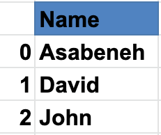
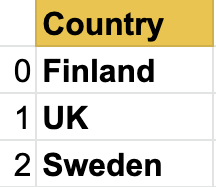
A series is a column and a DataFrame is a multidimensional table made up of collection of series. In order to create a pandas series we should use numpy to create a one dimensional arrays or a python list. Let us see an example of a series:
Names Pandas Series
Countries Series
Cities Series
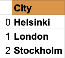
As you can see, pandas series is just one column of data. If we want to have multiple columns we use data frames. The example below shows pandas DataFrames.
Let us see, an example of a pandas data frame:
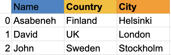
Data frame is a collection of rows and columns. Look at the table below; it has many more columns than the example above:
Next, we will see how to import pandas and how to create Series and DataFrames using pandas
Importing Pandas
import pandas as pd # importing pandas as pd
import numpy  as np # importing numpy as np
Creating Pandas Series with Default Index
nums = [1, 2, 3, 4,5]
s = pd.Series(nums)
print(s)
    0    1
    1    2
    2    3
    3    4
    4    5
    dtype: int64
Creating Pandas Series with custom index
nums = [1, 2, 3, 4, 5]
s = pd.Series(nums, index=[1, 2, 3, 4, 5])
print(s)
    1    1
    2    2
    3    3
    4    4
    5    5
    dtype: int64
fruits = ['Orange','Banana','Mango']
fruits = pd.Series(fruits, index=[1, 2, 3])
print(fruits)
    1    Orange
    2    Banana
    3    Mango
    dtype: object
Creating Pandas Series from a Dictionary
dct = {'name':'Asabeneh','country':'Finland','city':'Helsinki'}
s = pd.Series(dct)
print(s)
    name       Asabeneh
    country     Finland
    city       Helsinki
    dtype: object
Creating a Constant Pandas Series
s = pd.Series(10, index = [1, 2, 3])
print(s)
    1    10
    2    10
    3    10
    dtype: int64
Creating a Pandas Series Using Linspace
s = pd.Series(np.linspace(5, 20, 10)) # linspace(starting, end, items)
print(s)
    0     5.000000
    1     6.666667
    2     8.333333
    3    10.000000
    4    11.666667
    5    13.333333
    6    15.000000
    7    16.666667
    8    18.333333
    9    20.000000
    dtype: float64
DataFrames
Pandas data frames can be created in different ways.
Creating DataFrames from List of Lists
data = [
    ['Asabeneh', 'Finland', 'Helsink'],
    ['David', 'UK', 'London'],
    ['John', 'Sweden', 'Stockholm']
]
df = pd.DataFrame(data, columns=['Names','Country','City'])
print(df)
Creating DataFrame Using Dictionary
data = {'Name': ['Asabeneh', 'David', 'John'], 'Country':[
    'Finland', 'UK', 'Sweden'], 'City': ['Helsiki', 'London', 'Stockholm']}
df = pd.DataFrame(data)
print(df)
Creating DataFrames from a List of Dictionaries
data = [
    {'Name': 'Asabeneh', 'Country': 'Finland', 'City': 'Helsinki'},
    {'Name': 'David', 'Country': 'UK', 'City': 'London'},
    {'Name': 'John', 'Country': 'Sweden', 'City': 'Stockholm'}]
df = pd.DataFrame(data)
print(df)
Reading CSV File Using Pandas
To download the CSV file, what is needed in this example, console/command line is enough:
curl -O https://raw.githubusercontent.com/Asabeneh/30-Days-Of-Python/master/data/weight-height.csv
Put the downloaded file in your working directory.
import pandas as pd

df = pd.read_csv('weight-height.csv')
print(df)
Data Exploration
Let us read only the first 5 rows using head()
print(df.head()) # give five rows we can increase the number of rows by passing argument to the head() method
Let us also explore the last recordings of the dataframe using the tail() methods.
print(df.tail()) # tails give the last five rows, we can increase the rows by passing argument to tail method
As you can see the csv file has three rows: Gender, Height and Weight. If the DataFrame would have a long rows, it would be hard to know all the columns. Therefore, we should use a method to know the columns. we do not know the number of rows. Let's use shape method.
print(df.shape) # as you can see 10000 rows and three columns
(10000, 3)
Let us get all the columns using columns.
print(df.columns)
Index(['Gender', 'Height', 'Weight'], dtype='object')
Now, let us get a specific column using the column key
heights = df['Height'] # this is now a series
print(heights)
    0       73.847017
    1       68.781904
    2       74.110105
    3       71.730978
    4       69.881796
              ...
    9995    66.172652
    9996    67.067155
    9997    63.867992
    9998    69.034243
    9999    61.944246
    Name: Height, Length: 10000, dtype: float64
weights = df['Weight'] # this is now a series
print(weights)
    0       241.893563
    1       162.310473
    2       212.740856
    3       220.042470
    4       206.349801
               ...
    9995    136.777454
    9996    170.867906
    9997    128.475319
    9998    163.852461
    9999    113.649103
    Name: Weight, Length: 10000, dtype: float64
print(len(heights) == len(weights))
True
The describe() method provides a descriptive statistical values of a dataset.
print(heights.describe()) # give statistical information about height data
    count    10000.000000
    mean        66.367560
    std          3.847528
    min         54.263133
    25%         63.505620
    50%         66.318070
    75%         69.174262
    max         78.998742
    Name: Height, dtype: float64
print(weights.describe())
    count    10000.000000
    mean       161.440357
    std         32.108439
    min         64.700127
    25%        135.818051
    50%        161.212928
    75%        187.169525
    max        269.989699
    Name: Weight, dtype: float64
print(df.describe()) # describe can also give statistical information from a dataFrame
Similar to describe(), the info() method also give information about the dataset.
Modifying a DataFrame
Modifying a DataFrame: * We can create a new DataFrame * We can create a new column and add it to the DataFrame, * we can remove an existing column from a DataFrame, * we can modify an existing column in a DataFrame, * we can change the data type of column values in the DataFrame
Creating a DataFrame
As always, first we import the necessary packages. Now, lets import pandas and numpy, two best friends ever.
import pandas as pd
import numpy as np
data = [
    {"Name": "Asabeneh", "Country":"Finland","City":"Helsinki"},
    {"Name": "David", "Country":"UK","City":"London"},
    {"Name": "John", "Country":"Sweden","City":"Stockholm"}]
df = pd.DataFrame(data)
print(df)
Adding a column to a DataFrame is like adding a key to a dictionary.
First let's use the previous example to create a DataFrame. After we create the DataFrame, we will start modifying the columns and column values.
Adding a New Column
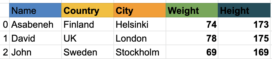
Let's add a weight column in the DataFrame
weights = [74, 78, 69]
df['Weight'] = weights
df
Let's add a height column into the DataFrame aswell
heights = [173, 175, 169]
df['Height'] = heights
print(df)
As you can see in the DataFrame above, we did add new columns, Weight and Height. Let's add one additional column called BMI(Body Mass Index) by calculating their BMI using thier mass and height. BMI is mass divided by height squared (in meters) - Weight/Height * Height.
As you can see, the height is in centimeters, so we shoud change it to meters. Let's modify the height row.
Modifying column values
df['Height'] = df['Height'] * 0.01
df
# Using functions makes our code clean, but you can calculate the bmi without one
def calculate_bmi ():
    weights = df['Weight']
    heights = df['Height']
    bmi = []
    for w,h in zip(weights, heights):
        b = w/(h*h)
        bmi.append(b)
    return bmi

bmi = calculate_bmi()
df['BMI'] = bmi
df
Formatting DataFrame columns
The BMI column values of the DataFrame are float with many significant digits after decimal. Let's change it to one significant digit after point.
df['BMI'] = round(df['BMI'], 1)
print(df)
The information in the DataFrame seems not yet complete, let's add birth year and current year columns.
birth_year = ['1769', '1985', '1990']
current_year = pd.Series(2020, index=[0, 1,2])
df['Birth Year'] = birth_year
df['Current Year'] = current_year
df
Checking data types of Column values
print(df.Weight.dtype)
dtype('int64')
df['Birth Year'].dtype # it gives string object , we should change this to number
df['Birth Year'] = df['Birth Year'].astype('int')
print(df['Birth Year'].dtype) # let's check the data type now
dtype('int32')
Now same for the current year:
df['Current Year'] = df['Current Year'].astype('int')
df['Current Year'].dtype
dtype('int32')
Now, the column values of birth year and current year are integers. We can calculate the age.
ages = df['Current Year'] - df['Birth Year']
ages
0    251
1     35
2     30
dtype: int32
df['Ages'] = ages
print(df)
The person in the first row lived so far for 251 years. It is unlikely for someone to live so long. Either it is a typo or the data is cooked. So lets fill that data with average of the columns without including outlier.
mean = (35 + 30)/ 2
mean = (35 + 30)/ 2
print('Mean: ',mean)	#it is good to add some description to the output, so we know what is what
Mean: 32.5
Boolean Indexing
print(df[df['Ages'] > 120])
print(df[df['Ages'] < 120])
Exercises: Day 25
- Read the hacker_news.csv file from data directory
- Get the first five rows
- Get the last five rows
- Get the title column as pandas series
- Count the number of rows and columns
- Filter the titles which contain python
- Filter the titles which contain JavaScript
- Explore the data and make sense of it
🎉 CONGRATULATIONS ! 🎉